Access Sentinel 2 Analysis Ready Data from Digital Earth Africa¶

https://explorer.digitalearth.africa/products/s2_l2a

Import Required Packages¶

[1]:

from pystac_client import Client

from odc.stac import configure_rio, stac_load

Set Collection Configuration¶

The configuration dictionary is determined from the product’s definition, available at https://explorer.digitalearth.africa/products/s2_l2a#definition-doc

All assets except SCL have the same configuration. SCL uses uint8 rather than uint16.

In the configuration, we also supply the aliases for each band. This means we can load data by band name rather than band number.

[2]:

config = {
    "s2_l2a": {
        "assets": {
            "*": {
                "data_type": "uint16",
                "nodata": 0,
                "unit": "1",
            },
            "SCL": {
                "data_type": "uint8",
                "nodata": 0,
                "unit": "1",
            },
        },
        "aliases": {
            "costal_aerosol": "B01",
            "blue": "B02",
            "green": "B03",
            "red": "B04",
            "red_edge_1": "B05",
            "red_edge_2": "B06",
            "red_edge_3": "B07",
            "nir": "B08",
            "nir_narrow": "B08A",
            "water_vapour": "B09",
            "swir_1": "B11",
            "swir_2": "B12",
            "mask": "SCL",
            "aerosol_optical_thickness": "AOT",
            "scene_average_water_vapour": "WVP",
        },
    }
}

Set AWS Configuration¶

Digital Earth Africa data is stored on S3 in Cape Town, Africa. To load the data, we must configure rasterio with the appropriate AWS S3 endpoint. This can be done with the odc.stac.configure_rio function. Documentation for this function is available at https://odc-stac.readthedocs.io/en/latest/_api/odc.stac.configure_rio.html#odc.stac.configure_rio.

The configuration below must be used when loading any Digital Earth Africa data through the STAC API.

[3]:

configure_rio(
    cloud_defaults=True,
    aws={"aws_unsigned": True},
    AWS_S3_ENDPOINT="s3.af-south-1.amazonaws.com",
)

Connect to the Digital Earth Africa STAC Catalog¶

[4]:

# Open the stac catalogue
catalog = Client.open("https://explorer.digitalearth.africa/stac")

Find STAC Items to Load¶

Define query parameters¶

[5]:

# Set a bounding box
# [xmin, ymin, xmax, ymax] in latitude and longitude
bbox = [37.76, 12.49, 37.77, 12.50]

# Set a start and end date
start_date = "2020-09-01"
end_date = "2020-12-01"

# Set the STAC collections
collections = ["s2_l2a"]

Construct query and get items from catalog¶

[6]:

# Build a query with the set parameters
query = catalog.search(
    bbox=bbox, collections=collections, datetime=f"{start_date}/{end_date}"
)

# Search the STAC catalog for all items matching the query
items = list(query.items())
print(f"Found: {len(items):d} datasets")

Found: 34 datasets

Load the Data¶

In this step, we specify the desired coordinate system, resolution (here 20m), and bands to load. We also pass the bounding box to the stac_load function to only load the requested data. Since the band aliases are contained in the config dictionary, bands can be loaded using these aliaes (e.g. "red" instead of "B04" below).

The data will be lazy-loaded with dask, meaning that is won’t be loaded into memory until necessary, such as when it is displayed.

[7]:

crs = "EPSG:6933"
resolution = 20

ds = stac_load(
    items,
    bands=("red", "green", "blue", "nir"),
    crs=crs,
    resolution=resolution,
    chunks={},
    groupby="solar_day",
    stac_cfg=config,
    bbox=bbox,
)

# View the Xarray Dataset
ds

[7]:

<xarray.Dataset> Size: 421kB
Dimensions:      (y: 63, x: 49, time: 17)
Coordinates:
  * y            (y) float64 504B 1.582e+06 1.582e+06 ... 1.581e+06 1.581e+06
  * x            (x) float64 392B 3.643e+06 3.643e+06 ... 3.644e+06 3.644e+06
    spatial_ref  int32 4B 6933
  * time         (time) datetime64[ns] 136B 2020-09-03T08:06:43 ... 2020-11-2...
Data variables:
    red          (time, y, x) uint16 105kB dask.array<chunksize=(1, 63, 49), meta=np.ndarray>
    green        (time, y, x) uint16 105kB dask.array<chunksize=(1, 63, 49), meta=np.ndarray>
    blue         (time, y, x) uint16 105kB dask.array<chunksize=(1, 63, 49), meta=np.ndarray>
    nir          (time, y, x) uint16 105kB dask.array<chunksize=(1, 63, 49), meta=np.ndarray>

Compute a band index¶

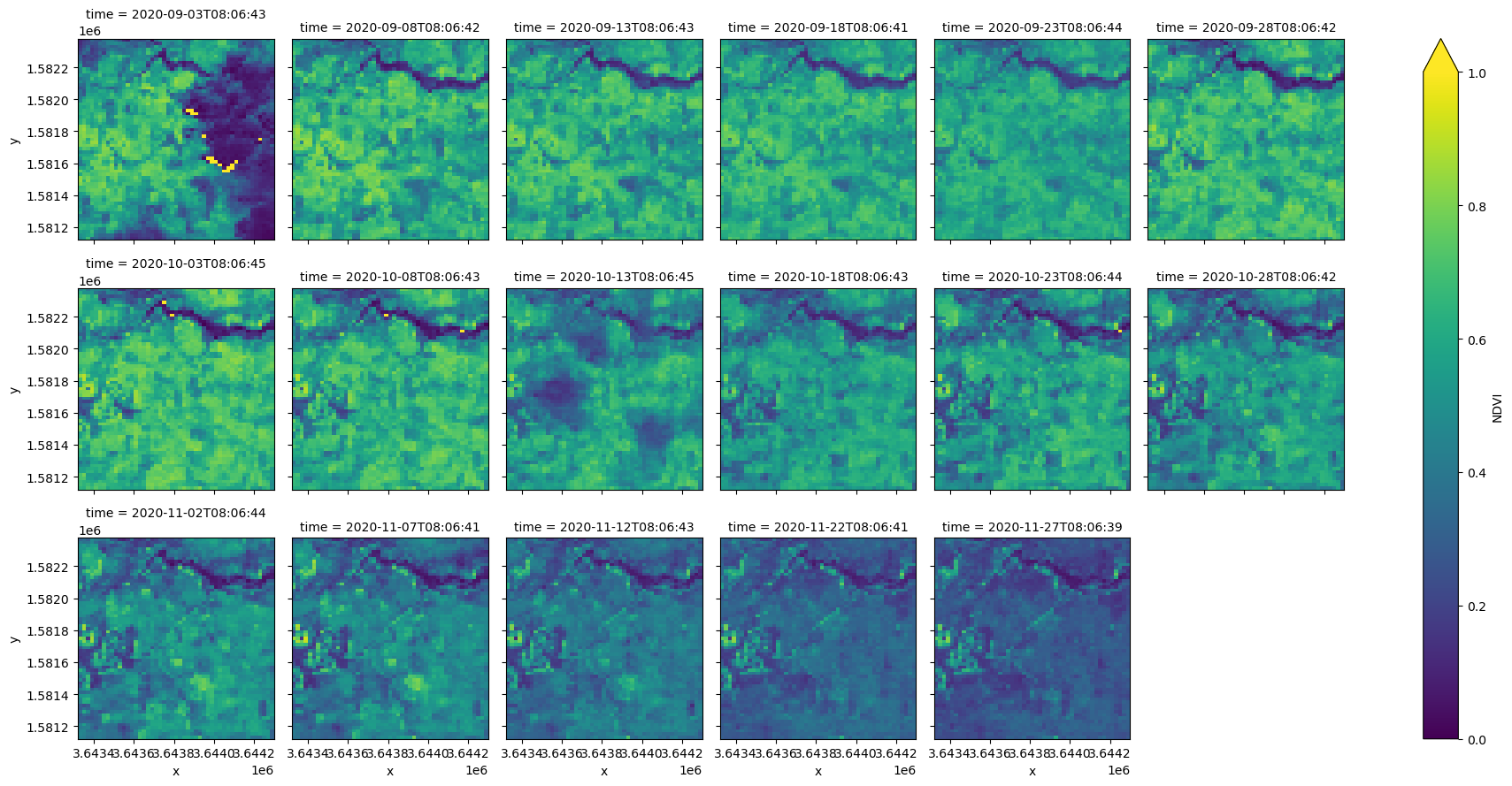
After loading the data, you can perform standard Xarray operations, such as calculating and plotting the normalised difference vegetation index (NDVI). The .compute() method triggers Dask to load the data into memory, so running this step may take a few minutes.

[8]:

ds["NDVI"] = (ds.nir - ds.red) / (ds.nir + ds.red)

ds.NDVI.compute().plot(col="time", col_wrap=6, vmin=0, vmax=1)

[8]:

<xarray.plot.facetgrid.FacetGrid at 0x7f77d74c6410>

../_images/notebooks_stac-load-S2-deafrica_16_1.png