Access Sentinel 2 Data from AWS
![]()
https://registry.opendata.aws/sentinel-2-l2a-cogs/
[1]:
import dask.distributed
import folium
import folium.plugins
import geopandas as gpd
import shapely.geometry
from IPython.display import display
from pystac_client import Client

from odc.stac import configure_rio, stac_load


def convert_bounds(bbox, invert_y=False):
    """
    Helper method for changing bounding box representation to leaflet notation

    ``(lon1, lat1, lon2, lat2) -> ((lat1, lon1), (lat2, lon2))``
    """
    x1, y1, x2, y2 = bbox
    if invert_y:
        y1, y2 = y2, y1
    return ((y1, x1), (y2, x2))
Start Dask Client
This step is optional, but it does improve load speed significantly. You don’t have to use Dask, as you can load data directly into memory of the notebook.
[2]:
client = dask.distributed.Client()
configure_rio(cloud_defaults=True, aws={"aws_unsigned": True}, client=client)
display(client)
Client
Client-c8cfcd3b-5016-11f1-8952-0022488e1f6f
| Connection method: Cluster object | Cluster type: distributed.LocalCluster |
| Dashboard: http://127.0.0.1:8787/status |
Cluster Info
LocalCluster
259c8ac7
| Dashboard: http://127.0.0.1:8787/status | Workers: 4 |
| Total threads: 4 | Total memory: 15.61 GiB |
| Status: running | Using processes: True |
Scheduler Info
Scheduler
Scheduler-3290f560-e76e-4888-847f-5441ab9d8bb3
| Comm: tcp://127.0.0.1:36771 | Workers: 0 |
| Dashboard: http://127.0.0.1:8787/status | Total threads: 0 |
| Started: Just now | Total memory: 0 B |
Workers
Worker: 0
| Comm: tcp://127.0.0.1:43497 | Total threads: 1 |
| Dashboard: http://127.0.0.1:36723/status | Memory: 3.90 GiB |
| Nanny: tcp://127.0.0.1:43203 | |
| Local directory: /tmp/dask-scratch-space/worker-f6qa795z | |
Worker: 1
| Comm: tcp://127.0.0.1:34273 | Total threads: 1 |
| Dashboard: http://127.0.0.1:45871/status | Memory: 3.90 GiB |
| Nanny: tcp://127.0.0.1:42395 | |
| Local directory: /tmp/dask-scratch-space/worker-erzd2841 | |
Worker: 2
| Comm: tcp://127.0.0.1:41823 | Total threads: 1 |
| Dashboard: http://127.0.0.1:38149/status | Memory: 3.90 GiB |
| Nanny: tcp://127.0.0.1:41767 | |
| Local directory: /tmp/dask-scratch-space/worker-36wvd_fm | |
Worker: 3
| Comm: tcp://127.0.0.1:33913 | Total threads: 1 |
| Dashboard: http://127.0.0.1:40001/status | Memory: 3.90 GiB |
| Nanny: tcp://127.0.0.1:33279 | |
| Local directory: /tmp/dask-scratch-space/worker-dkq95g7w | |
Find STAC Items to Load
[3]:
km2deg = 1.0 / 111
x, y = (113.887, -25.843)  # Center point of a query
r = 100 * km2deg
bbox = (x - r, y - r, x + r, y + r)

catalog = Client.open("https://earth-search.aws.element84.com/v1/")

query = catalog.search(
    collections=["sentinel-2-l2a"], datetime="2021-09-16", limit=100, bbox=bbox
)

items = list(query.items())
print(f"Found: {len(items):d} datasets")

# Convert STAC items into a GeoJSON FeatureCollection
stac_json = query.item_collection_as_dict()
Found: 18 datasets
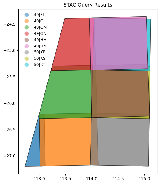
Review Query Result
We’ll use GeoPandas DataFrame object to make plotting easier.
[4]:
gdf = gpd.GeoDataFrame.from_features(stac_json, "epsg:4326")

# Compute granule id from components
gdf["granule"] = (
    gdf["mgrs:utm_zone"].apply(lambda x: f"{x:02d}")
    + gdf["mgrs:latitude_band"]
    + gdf["mgrs:grid_square"]
)

fig = gdf.plot(
    "granule",
    edgecolor="black",
    categorical=True,
    aspect="equal",
    alpha=0.5,
    figsize=(6, 12),
    legend=True,
    legend_kwds={"loc": "upper left", "frameon": False, "ncol": 1},
)
_ = fig.set_title("STAC Query Results")
Plot STAC Items on a Map
[5]:
# https://github.com/python-visualization/folium/issues/1501
from branca.element import Figure

fig = Figure(width="400px", height="500px")
map1 = folium.Map()
fig.add_child(map1)

folium.GeoJson(
    shapely.geometry.box(*bbox),
    style_function=lambda x: dict(fill=False, weight=1, opacity=0.7, color="olive"),
    name="Query",
).add_to(map1)

gdf.explore(
    "granule",
    categorical=True,
    tooltip=[
        "granule",
        "datetime",
        "eo:cloud_cover",
    ],
    popup=True,
    style_kwds=dict(fillOpacity=0.1, width=2),
    name="STAC",
    m=map1,
)

map1.fit_bounds(bounds=convert_bounds(gdf.unary_union.bounds))
display(fig)
/tmp/ipykernel_2386/1652784297.py:28: DeprecationWarning: The 'unary_union' attribute is deprecated, use the 'union_all()' method instead.
  map1.fit_bounds(bounds=convert_bounds(gdf.unary_union.bounds))
Construct Dask Dataset
Note that even though there are 9 STAC Items on input, there is only one timeslice on output. This is because of groupby="solar_day". With that setting stac_load will place all items that occured on the same day (as adjusted for the timezone) into one image plane.
[6]:
# Since we will plot it on a map we need to use `EPSG:3857` projection
crs = "epsg:3857"
zoom = 2**5  # overview level 5

xx = stac_load(
    items,
    bands=("red", "green", "blue"),
    crs=crs,
    resolution=10 * zoom,
    chunks={},  # <-- use Dask
    groupby="solar_day",
)
display(xx)
<xarray.Dataset> Size: 7MB
Dimensions:      (y: 1101, x: 1087, time: 1)
Coordinates:
  * y            (y) float64 9kB -2.797e+06 -2.798e+06 ... -3.149e+06 -3.149e+06
  * x            (x) float64 9kB 1.247e+07 1.247e+07 ... 1.282e+07 1.282e+07
    spatial_ref  int32 4B 3857
  * time         (time) datetime64[ns] 8B 2021-09-16T02:34:44.451000
Data variables:
    red          (time, y, x) uint16 2MB dask.array<chunksize=(1, 1101, 1087), meta=np.ndarray>
    green        (time, y, x) uint16 2MB dask.array<chunksize=(1, 1101, 1087), meta=np.ndarray>
blue (time, y, x) uint16 2MB dask.array<chunksize=(1, 1101, 1087), meta=np.ndarray>Note that data is not loaded yet. But we can review memory requirement. We can also check data footprint.
[7]:
xx.odc.geobox
[7]:
GeoBox
WKT
BASEGEOGCRS["WGS 84",
DATUM["World Geodetic System 1984",
ELLIPSOID["WGS 84",6378137,298.257223563,
LENGTHUNIT["metre",1]]],
PRIMEM["Greenwich",0,
ANGLEUNIT["degree",0.0174532925199433]],
ID["EPSG",4326]],
CONVERSION["unnamed",
METHOD["Popular Visualisation Pseudo Mercator",
ID["EPSG",1024]],
PARAMETER["Latitude of natural origin",0,
ANGLEUNIT["degree",0.0174532925199433],
ID["EPSG",8801]],
PARAMETER["Longitude of natural origin",0,
ANGLEUNIT["degree",0.0174532925199433],
ID["EPSG",8802]],
PARAMETER["False easting",0,
LENGTHUNIT["metre",1],
ID["EPSG",8806]],
PARAMETER["False northing",0,
LENGTHUNIT["metre",1],
ID["EPSG",8807]]],
CS[Cartesian,2],
AXIS["easting (X)",east,
ORDER[1],
LENGTHUNIT["metre",1]],
AXIS["northing (Y)",north,
ORDER[2],
LENGTHUNIT["metre",1]],
USAGE[
SCOPE["Web mapping and visualisation."],
AREA["World between 85.06°S and 85.06°N."],
BBOX[-85.06,-180,85.06,180]],
ID["EPSG",3857]]
Load data into local memory
[8]:
%%time
xx = xx.compute()
CPU times: user 518 ms, sys: 80.4 ms, total: 598 ms
Wall time: 10.9 s
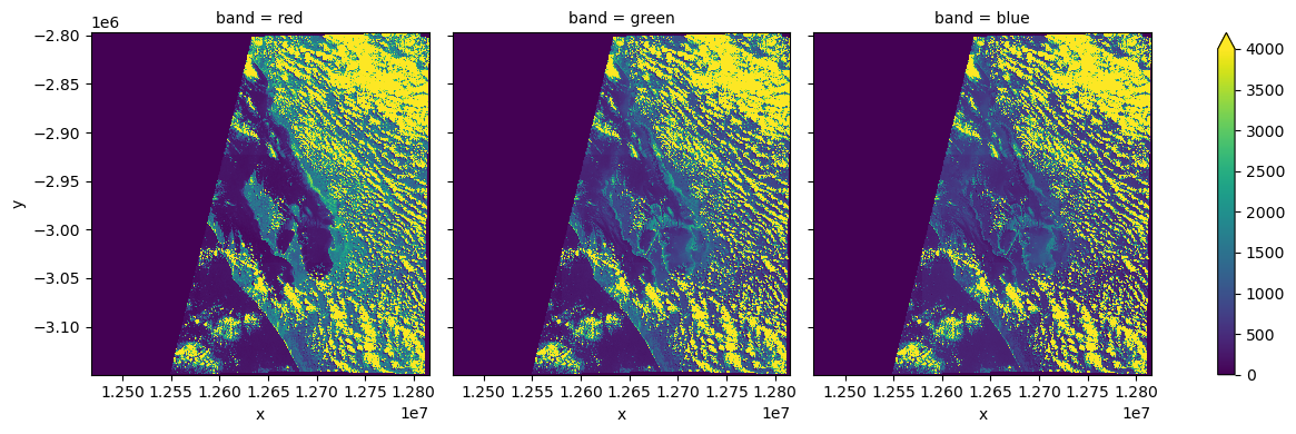
[9]:
_ = (
    xx.isel(time=0)
    .to_array("band")
    .plot.imshow(
        col="band",
        size=4,
        vmin=0,
        vmax=4000,
    )
)
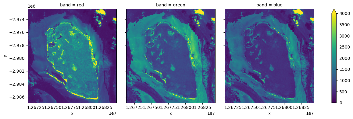
Load with bounding box
As you can see stac_load returned all the data covered by STAC items returned from the query. This happens by default as stac_load has no way of knowing what your query was. But it is possible to control what region is loaded. There are several mechanisms available, but probably simplest one is to use bbox= parameter (compatible with stac_client).
Let’s load a small region at native resolution to demonstrate.
[10]:
r = 6.5 * km2deg
small_bbox = (x - r, y - r, x + r, y + r)

yy = stac_load(
    items,
    bands=("red", "green", "blue"),
    crs=crs,
    resolution=10,
    chunks={},  # <-- use Dask
    groupby="solar_day",
    bbox=small_bbox,
)
display(yy.odc.geobox)
GeoBox
WKT
BASEGEOGCRS["WGS 84",
DATUM["World Geodetic System 1984",
ELLIPSOID["WGS 84",6378137,298.257223563,
LENGTHUNIT["metre",1]]],
PRIMEM["Greenwich",0,
ANGLEUNIT["degree",0.0174532925199433]],
ID["EPSG",4326]],
CONVERSION["unnamed",
METHOD["Popular Visualisation Pseudo Mercator",
ID["EPSG",1024]],
PARAMETER["Latitude of natural origin",0,
ANGLEUNIT["degree",0.0174532925199433],
ID["EPSG",8801]],
PARAMETER["Longitude of natural origin",0,
ANGLEUNIT["degree",0.0174532925199433],
ID["EPSG",8802]],
PARAMETER["False easting",0,
LENGTHUNIT["metre",1],
ID["EPSG",8806]],
PARAMETER["False northing",0,
LENGTHUNIT["metre",1],
ID["EPSG",8807]]],
CS[Cartesian,2],
AXIS["easting (X)",east,
ORDER[1],
LENGTHUNIT["metre",1]],
AXIS["northing (Y)",north,
ORDER[2],
LENGTHUNIT["metre",1]],
USAGE[
SCOPE["Web mapping and visualisation."],
AREA["World between 85.06°S and 85.06°N."],
BBOX[-85.06,-180,85.06,180]],
ID["EPSG",3857]]
[11]:
yy = yy.compute()
[12]:
_ = (
    yy.isel(time=0)
    .to_array("band")
    .plot.imshow(
        col="band",
        size=4,
        vmin=0,
        vmax=4000,
    )
)