Access Sentinel 2 Data on Planetary Computer
![]()
Setup Instructions
This notebook is meant to run on Planetary Computer lab hub.
[1]:
import dask.distributed
import dask.utils
import numpy as np
import planetary_computer as pc
import xarray as xr
from IPython.display import display
from pystac_client import Client

from odc.stac import configure_rio, stac_load
Start Dask Client
This step is optional, but it does improve load speed significantly. You don’t have to use Dask, as you can load data directly into memory of the notebook.
[2]:
client = dask.distributed.Client()
configure_rio(cloud_defaults=True, client=client)
display(client)
Client
Client-da12c186-5016-11f1-89b4-0022488e1f6f
| Connection method: Cluster object | Cluster type: distributed.LocalCluster |
| Dashboard: http://127.0.0.1:8787/status |
Cluster Info
LocalCluster
f0cc0a9d
| Dashboard: http://127.0.0.1:8787/status | Workers: 4 |
| Total threads: 4 | Total memory: 15.61 GiB |
| Status: running | Using processes: True |
Scheduler Info
Scheduler
Scheduler-2e6a9455-91bc-468f-a7ec-3634faba4246
| Comm: tcp://127.0.0.1:33761 | Workers: 0 |
| Dashboard: http://127.0.0.1:8787/status | Total threads: 0 |
| Started: Just now | Total memory: 0 B |
Workers
Worker: 0
| Comm: tcp://127.0.0.1:40023 | Total threads: 1 |
| Dashboard: http://127.0.0.1:33101/status | Memory: 3.90 GiB |
| Nanny: tcp://127.0.0.1:42387 | |
| Local directory: /tmp/dask-scratch-space/worker-b4tab01z | |
Worker: 1
| Comm: tcp://127.0.0.1:45275 | Total threads: 1 |
| Dashboard: http://127.0.0.1:44955/status | Memory: 3.90 GiB |
| Nanny: tcp://127.0.0.1:39179 | |
| Local directory: /tmp/dask-scratch-space/worker-9rq_21zw | |
Worker: 2
| Comm: tcp://127.0.0.1:39703 | Total threads: 1 |
| Dashboard: http://127.0.0.1:43327/status | Memory: 3.90 GiB |
| Nanny: tcp://127.0.0.1:43147 | |
| Local directory: /tmp/dask-scratch-space/worker-oaxl7jxf | |
Worker: 3
| Comm: tcp://127.0.0.1:34999 | Total threads: 1 |
| Dashboard: http://127.0.0.1:36139/status | Memory: 3.90 GiB |
| Nanny: tcp://127.0.0.1:45949 | |
| Local directory: /tmp/dask-scratch-space/worker-4xqovevs | |
Query STAC API
Here we are looking for datasets in sentinel-2-l2a collection from June 2019 over MGRS tile 06VVN.
[3]:
catalog = Client.open("https://planetarycomputer.microsoft.com/api/stac/v1")

query = catalog.search(
    collections=["sentinel-2-l2a"],
    datetime="2019-06",
    query={"s2:mgrs_tile": dict(eq="06VVN")},
)

items = list(query.items())
print(f"Found: {len(items):d} datasets")
Found: 23 datasets
Lazy load all the bands
We won’t use all the bands but it doesn’t matter as bands that we won’t use won’t be loaded. We are “loading” data with Dask, which means that at this point no reads will be happening just yet.
We have to supply dtype= and nodata= because items in this collection are missing raster extension metadata.
[4]:
resolution = 10
SHRINK = 4
if client.cluster.workers[0].memory_manager.memory_limit < dask.utils.parse_bytes("4G"):
    SHRINK = 8  # running on Binder with 2Gb RAM

if SHRINK > 1:
    resolution = resolution * SHRINK

xx = stac_load(
    items,
    chunks={"x": 2048, "y": 2048},
    patch_url=pc.sign,
    resolution=resolution,
    # force dtype and nodata
    dtype="uint16",
    nodata=0,
)

print(f"Bands: {','.join(list(xx.data_vars))}")
display(xx)
Bands: AOT,B01,B02,B03,B04,B05,B06,B07,B08,B09,B11,B12,B8A,SCL,WVP,visual
<xarray.Dataset> Size: 6GB
Dimensions:      (y: 2745, x: 2745, time: 23)
Coordinates:
  * y            (y) float64 22kB 6.8e+06 6.8e+06 6.8e+06 ... 6.69e+06 6.69e+06
  * x            (x) float64 22kB 4e+05 4e+05 4.001e+05 ... 5.097e+05 5.097e+05
    spatial_ref  int32 4B 32606
  * time         (time) datetime64[ns] 184B 2019-06-01T21:15:21.024000 ... 20...
Data variables: (12/16)
    AOT          (time, y, x) uint16 347MB dask.array<chunksize=(1, 2048, 2048), meta=np.ndarray>
    B01          (time, y, x) uint16 347MB dask.array<chunksize=(1, 2048, 2048), meta=np.ndarray>
    B02          (time, y, x) uint16 347MB dask.array<chunksize=(1, 2048, 2048), meta=np.ndarray>
    B03          (time, y, x) uint16 347MB dask.array<chunksize=(1, 2048, 2048), meta=np.ndarray>
    B04          (time, y, x) uint16 347MB dask.array<chunksize=(1, 2048, 2048), meta=np.ndarray>
    B05          (time, y, x) uint16 347MB dask.array<chunksize=(1, 2048, 2048), meta=np.ndarray>
    ...           ...
    B11          (time, y, x) uint16 347MB dask.array<chunksize=(1, 2048, 2048), meta=np.ndarray>
    B12          (time, y, x) uint16 347MB dask.array<chunksize=(1, 2048, 2048), meta=np.ndarray>
    B8A          (time, y, x) uint16 347MB dask.array<chunksize=(1, 2048, 2048), meta=np.ndarray>
    SCL          (time, y, x) uint16 347MB dask.array<chunksize=(1, 2048, 2048), meta=np.ndarray>
    WVP          (time, y, x) uint16 347MB dask.array<chunksize=(1, 2048, 2048), meta=np.ndarray>
visual (time, y, x) uint16 347MB dask.array<chunksize=(1, 2048, 2048), meta=np.ndarray>By default stac_load will return all the data bands using canonical asset names. But we can also request a subset of bands, by supplying bands= parameter. When going this route you can also use “common name” to refer to a band.
In this case we request red,green,blue,nir bands which are common names for bands B04,B03,B02,B08 and SCL band which is a canonical name.
[5]:
xx = stac_load(
    items,
    bands=["red", "green", "blue", "nir", "SCL"],
    resolution=resolution,
    chunks={"x": 2048, "y": 2048},
    patch_url=pc.sign,
    # force dtype and nodata
    dtype="uint16",
    nodata=0,
)

print(f"Bands: {','.join(list(xx.data_vars))}")
display(xx)
Bands: red,green,blue,nir,SCL
<xarray.Dataset> Size: 2GB
Dimensions:      (y: 2745, x: 2745, time: 23)
Coordinates:
  * y            (y) float64 22kB 6.8e+06 6.8e+06 6.8e+06 ... 6.69e+06 6.69e+06
  * x            (x) float64 22kB 4e+05 4e+05 4.001e+05 ... 5.097e+05 5.097e+05
    spatial_ref  int32 4B 32606
  * time         (time) datetime64[ns] 184B 2019-06-01T21:15:21.024000 ... 20...
Data variables:
    red          (time, y, x) uint16 347MB dask.array<chunksize=(1, 2048, 2048), meta=np.ndarray>
    green        (time, y, x) uint16 347MB dask.array<chunksize=(1, 2048, 2048), meta=np.ndarray>
    blue         (time, y, x) uint16 347MB dask.array<chunksize=(1, 2048, 2048), meta=np.ndarray>
    nir          (time, y, x) uint16 347MB dask.array<chunksize=(1, 2048, 2048), meta=np.ndarray>
SCL (time, y, x) uint16 347MB dask.array<chunksize=(1, 2048, 2048), meta=np.ndarray>Do some math with bands
[6]:
def to_float(xx):
    _xx = xx.astype("float32")
    nodata = _xx.attrs.pop("nodata", None)
    if nodata is None:
        return _xx
    return _xx.where(xx != nodata)


def colorize(xx, colormap):
    return xr.DataArray(colormap[xx.data], coords=xx.coords, dims=(*xx.dims, "band"))
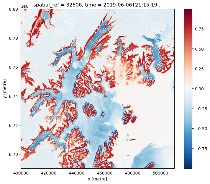
[7]:
# like .astype(float32) but taking care of nodata->NaN mapping
nir = to_float(xx.nir)
red = to_float(xx.red)
ndvi = (nir - red) / (
    nir + red
)  # < This is still a lazy Dask computation (no data loaded yet)

# Get the 5-th time slice `load->compute->plot`
_ = ndvi.isel(time=4).compute().plot.imshow(size=7, aspect=1.2, interpolation="bicubic")
For sample purposes work with first 6 observations only
[8]:
xx = xx.isel(time=np.s_[:6])
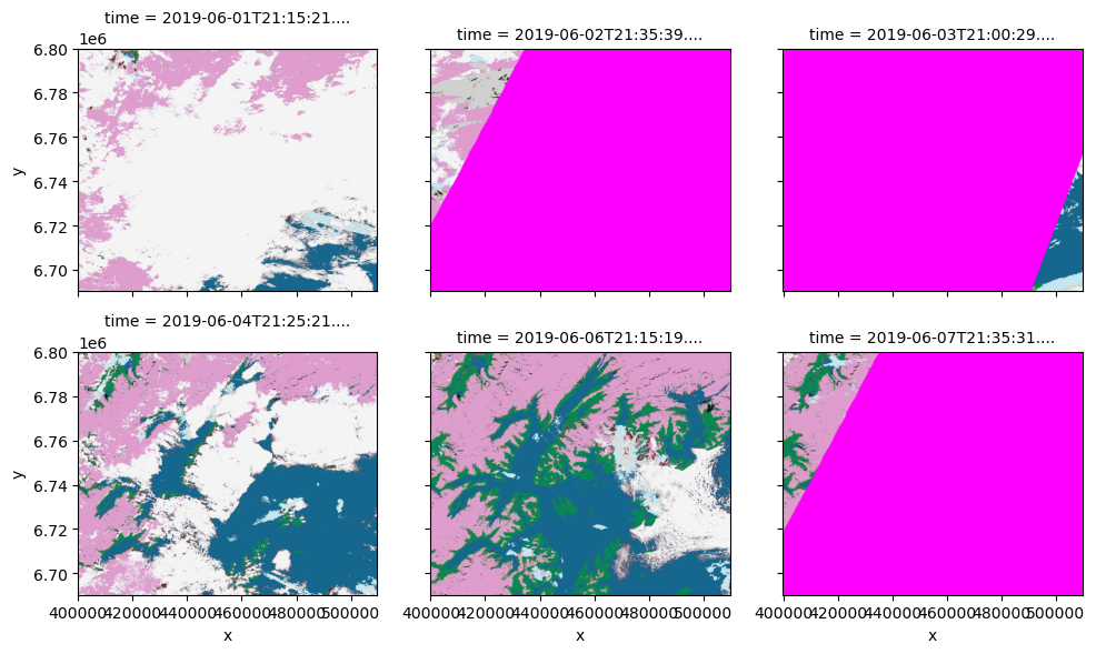
[9]:
# fmt: off
scl_colormap = np.array(
    [
        [255,   0, 255, 255],  # 0  - NODATA
        [255,   0,   4, 255],  # 1  - Saturated or Defective
        [0  ,   0,   0, 255],  # 2  - Dark Areas
        [97 ,  97,  97, 255],  # 3  - Cloud Shadow
        [3  , 139,  80, 255],  # 4  - Vegetation
        [192, 132,  12, 255],  # 5  - Bare Ground
        [21 , 103, 141, 255],  # 6  - Water
        [117,   0,  27, 255],  # 7  - Unclassified
        [208, 208, 208, 255],  # 8  - Cloud
        [244, 244, 244, 255],  # 9  - Definitely Cloud
        [195, 231, 240, 255],  # 10 - Thin Cloud
        [222, 157, 204, 255],  # 11 - Snow or Ice
    ],
    dtype="uint8",
)
# fmt: on

# Load SCL band, then convert to RGB using color scheme above
scl_rgba = colorize(xx.SCL.compute(), scl_colormap)

# Check we still have geo-registration
scl_rgba.odc.geobox
[9]:
GeoBox
WKT
BASEGEOGCRS["WGS 84",
ENSEMBLE["World Geodetic System 1984 ensemble",
MEMBER["World Geodetic System 1984 (Transit)"],
MEMBER["World Geodetic System 1984 (G730)"],
MEMBER["World Geodetic System 1984 (G873)"],
MEMBER["World Geodetic System 1984 (G1150)"],
MEMBER["World Geodetic System 1984 (G1674)"],
MEMBER["World Geodetic System 1984 (G1762)"],
MEMBER["World Geodetic System 1984 (G2139)"],
MEMBER["World Geodetic System 1984 (G2296)"],
ELLIPSOID["WGS 84",6378137,298.257223563,
LENGTHUNIT["metre",1]],
ENSEMBLEACCURACY[2.0]],
PRIMEM["Greenwich",0,
ANGLEUNIT["degree",0.0174532925199433]],
ID["EPSG",4326]],
CONVERSION["UTM zone 6N",
METHOD["Transverse Mercator",
ID["EPSG",9807]],
PARAMETER["Latitude of natural origin",0,
ANGLEUNIT["degree",0.0174532925199433],
ID["EPSG",8801]],
PARAMETER["Longitude of natural origin",-147,
ANGLEUNIT["degree",0.0174532925199433],
ID["EPSG",8802]],
PARAMETER["Scale factor at natural origin",0.9996,
SCALEUNIT["unity",1],
ID["EPSG",8805]],
PARAMETER["False easting",500000,
LENGTHUNIT["metre",1],
ID["EPSG",8806]],
PARAMETER["False northing",0,
LENGTHUNIT["metre",1],
ID["EPSG",8807]]],
CS[Cartesian,2],
AXIS["(E)",east,
ORDER[1],
LENGTHUNIT["metre",1]],
AXIS["(N)",north,
ORDER[2],
LENGTHUNIT["metre",1]],
USAGE[
SCOPE["Navigation and medium accuracy spatial referencing."],
AREA["Between 150°W and 144°W, northern hemisphere between equator and 84°N, onshore and offshore. United States (USA) - Alaska (AK)."],
BBOX[0,-150,84,-144]],
ID["EPSG",32606]]
[10]:
_ = scl_rgba.plot.imshow(col="time", col_wrap=3, size=3, interpolation="antialiased")
Let’s save image dated 2019-06-04 to a cloud optimized geotiff file.
[11]:
to_save = scl_rgba.isel(time=3)
fname = f"SCL-{to_save.time.dt.strftime('%Y%m%d').item()}.tif"
print(f"Saving to: '{fname}'")
Saving to: 'SCL-20190604.tif'
[12]:
scl_rgba.isel(time=3).odc.write_cog(
    fname,
    overwrite=True,
    compress="webp",
    webp_quality=90,
)
[12]:
PosixPath('SCL-20190604.tif')
Check the file with rio info.
[13]:
!ls -lh {fname}
!rio info {fname} | jq .
-rw-r--r-- 1 runner runner 1.4M May 15 04:31 SCL-20190604.tif
{
  "blockxsize": 512,
  "blockysize": 512,
  "bounds": [
    399960.0,
    6690240.0,
    509760.0,
    6800040.0
  ],
  "colorinterp": [
    "red",
    "green",
    "blue",
    "alpha"
  ],
  "compress": "webp",
  "count": 4,
  "crs": "EPSG:32606",
  "descriptions": [
    null,
    null,
    null,
    null
  ],
  "driver": "GTiff",
  "dtype": "uint8",
  "height": 2745,
  "indexes": [
    1,
    2,
    3,
    4
  ],
  "interleave": "pixel",
  "lnglat": [
    -147.83041488908293,
    60.83899713274621
  ],
  "mask_flags": [
    [
      "per_dataset",
      "alpha"
    ],
    [
      "per_dataset",
      "alpha"
    ],
    [
      "per_dataset",
      "alpha"
    ],
    [
      "all_valid"
    ]
  ],
  "nodata": null,
  "res": [
    40.0,
    40.0
  ],
  "shape": [
    2745,
    2745
  ],
  "tiled": true,
  "transform": [
    40.0,
    0.0,
    399960.0,
    0.0,
    -40.0,
    6800040.0,
    0.0,
    0.0,
    1.0
  ],
  "units": [
    null,
    null,
    null,
    null
  ],
  "width": 2745
}